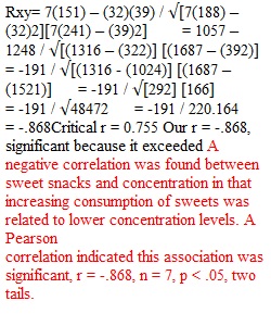
Q Psychology Statistics Dr. Robin Akawi Spring 2022 STATS PACK 3: WEEK 11 “Relationships and Expectations” Worksheets included: Concepts Page Length WEEK 10 Tech Practice 3 WEEK 11 Pearson Correlation 3 Intro to Regression Analyses (i.e., Prediction) 2 WEEK 12 Exam 2 WEEK 13 Intro to Chi Square 5 Statistical Software Outputs (Excel, Vassarstats) Open Statistical Software Outputs (SPSS if available) Open Pearson Correlation and Intro to Bivariate Regression “Are We Related?” Introducing you to variables that are related (associated) with each other, there are two kind of correlations to start with. Linear and curvilinear (non-linear). We will be focusing on the linear, which is analyzed with Pearson Correlation statistics. The letter used to note this is “r”. That is the correlation coefficient. There is also a type of correlation that is non-linear. Knowing this helps you ensure that you are using a Pearson Correlation when appropriate. Meaning, if you plot your data and notice a curved distribution it means you should not do Pearson. Let’s look at some visual examples. • Plot (a) shows a linear “positive” correlation in which as one variable’s values increase, so does the other variable’s values. You would also get this same linear line if as one variable’s values decrease, so does the other variable’s values. The one showing is a “strong” relationship with a value of +.82. • Plot (b) shows a linear “negative” correlation in which as one variable’s values increase, the other variable’s values decrease. You would also get this same linear line if as one variable’s values decrease, the other variable’s values increase. The one is also showing a “strong” relationship with a value of -.72. • Plot (c) is showing “no relationship”. The value this would get would be almost “0”. • Plot (d) is a curvilinear (non-linear) relationship. The value may be strong, but technically since it starts as a positive correlation then at some point switches directions into a negative correlation it is not appropriate for doing Pearson. So, this worksheet will focus on Plots a, b, and c. Examples of scenarios for data: (a) Studying and grades (b) Partying and grades (c) Favorite color and shoe size (d) Anxiety and performance A Scenario to Think About: Since we covered the effects of two levels of snacks (salty and sweet) with Factorial ANOVA and found varied results on the number of errors students made, let’s look at just the sweet snacks and how they relate to concentration. We gather two scores from each of our 7 students, the first score being the number sweet snacks they consumed yesterday, and the second score being them rating how well they felt they were able to concentrate yesterday. The “sweets” is our X variable and “concentration” is our Y variable. To keep you on track with the order of the steps, here are the specific instructions: • For each value in the X and Y columns, square each and put that value in the column to the right of it. For example, in the model on the previous page, the first score in the X column is 40. When you square that you get 1600 so that will go in the column to the right that is titled X2. After that you have the column titled “XY”. That means multiply each X value with each Y value. For example, in the model, that score of 40 for Student A should be multiplied with that student’s GPA of 3.75. That calculation equal 150 which goes in the last column. To the right, enter your N (sample size). • Next, add up each column to get the Sum of each (where you see each ? symbol). That is it for the pre-calculations. You are now ready to put them into the formula. Then follow the “order of operations” (PEMDAS) to finish out the calculation to get our Pearson r correlation coefficient measuring the relationship between x and y… which is why we note that as rxy. Student X(sweets) X2 Y(concentration) Y2 XY N A 6 4 B 3 5 C 2 7 D 5 6 E 7 5 F 8 3 G 1 9 ?X = ?X2 = ?Y = ?Y2= ?XY = Calculate the Pearson r (linear) Correlation Generate a basic scatter plot using either Excel or Google Sheets with our data and paste it below: For the remainder of this worksheet, answer the questions and see how we turn this correlation into a regression analysis. 1. You have the correlation value now. Determine the critical value that we would compare it to using an a = .05, two-tailed, and determine if the correlation is significant. See table below. Remember for correlation it is different for the df. Even though it’s one group of individuals we do not use n-1. Since each person has two types of scores, use n-2. Critical r = Our r = 2. Write out how you would describe the correlation in a publication. Be sure to include the description as well as the values and noting if the results were significant or not. 3. If you were talking to a friend who wants to eat snacks while doing course work in order to concentrate, note what you would say based on the results you obtained with this correlation? 4. There is a way to predict your concentration levels based on how many sweets you eat. Let’s do a bivariate regression analysis. Bivariate means two (bi) variables (variate). Let’s start with the correlation calculations you did early and just add two columns. Bring all the info down from the earlier table and do the last two column calculations. N X(sweets) X2 Y(concentration) Y2 XY (X-MX)2 (Y-MY)2 A 6 4 B 3 5 C 2 7 D 5 6 E 7 5 F 8 3 G 1 9 N=7 ?X = 32 MX = 4.57 ?X2 = ?Y = 39 MY = 5.57 ?Y2= ?XY = SSX = SSY = 5. Figure the linear prediction rule… i.e., the slope (b) and intercept (a) with the following formulas. 6. Write out the regression formula based on the results from #5. Predicted Y = a + bX Predicted Y = 7. Calculate the predicted salaries based on the following GPA scores: 1.00 and 9.00 Predicted Y = Predicted Y = 8. Copy the scatterplot from the correlation section and paste (or draw) here. Plot the two dots that will help draw the regression line… Dot 1 … X = 1 and Y = the first predicted Y value you calculated in #7 Dot 2 … X = 9 and Y = the second predicted Y value you calculated in #7 Draw a line connecting those two dots. THAT is your regression line that allows you to predict scores. Remember to correctly label each axis. 9. What would the predicted concentration level if consuming 3 sweets? What would the predicted concentration level if consuming 7 sweets? 10. Figure the standardized regression coefficient. ? = 11. Explain the logic of doing what you did in #5… i.e., why might this be important to do? Hint: Why do we standardize any scores in general? 12. Do you notice something similar between our ? we calculated here and the r we calculated earlier for the Pearson correlation? They are the same value! ? What we also know is that when we do a correlation coefficient in many statistical programs, it will give us the “effect size” for this association and prediction. It is called r2. For this last item, do the following: In this bivariate regression analysis, calculate the ?2 (or you can think of it as r2) and enter that value in the following sentence… followed by drawing a Venn Diagram to illustrate the overlap of the two variables. Be sure to label the X circle and the Y circle (which are the two variables) and put the r2 value in the part of the diagram that overlaps. ? = r = r2 = (Double check with Vassarstats) Paste results below. Statement of the effect size: Results show that _____% of the variation in our concentration levels can be attributed to how many sweets we consume while doing coursework. This is interesting because if sweets consumed account for that amount listed above, that must mean that approximately _____% must be due to something else. Name one other major factor that you think may be that “other” contributing factor. ________________ (There is really not a “right” answer here. You just need to be logical in noting what can affect your concentration in addition to the food you eat.)
View Related Questions